What decades of networking and distributed systems engineering can teach us about AI inference

The models are new. Many of the constraints are familiar.

A GPU can stay busy while the service around it gets slower. A smaller weight file can leave too little memory for the requests you need to serve. Separating a workload across machines can save compute and add enough communication to erase the gain.

Choosing a better model will not, on its own, solve these problems.

Scheduling, numerical representation, caching and distributed execution are familiar territory for systems engineers. Adapting that work to autoregressive models takes substantial engineering, but it gives teams a useful place to start. Find the resource that limits the service, then check whether an optimization helps requests finish sooner or at a lower cost.

Continuous batching is a scheduling problem

A serving batch might contain a short reply alongside a long explanation. If the system holds that batch together until every request finishes, completed requests leave capacity that new arrivals cannot immediately use. Orca's 2022 paper addressed this with iteration-level scheduling: the scheduler chooses the requests for each model iteration rather than fixing the batch for their entire lifetimes.1

This is the scheduling idea behind continuous batching. The scheduler can retire finished work and admit new work between iterations.1

Earlier server designs faced similar scheduling constraints. SEDA organized internet services into stages connected by explicit queues, with resource controllers to manage changing load.10 Both designs give the system explicit control over pending work and resource allocation. The comparison helps explain the design problem; it does not establish that Orca descended from SEDA.

A decoding sequence also has requirements that a packet or event does not. An active LLM request retains attention state across iterations, so admission decisions must account for memory as well as execution capacity.1

Keeping the GPU occupied is only part of the job. A batch policy must also protect latency as prompt and output lengths change. Admitting more work can improve aggregate throughput while making each user wait longer. Orca explicitly treats maximum batch size as a throughput-versus-latency control.1

Test the scheduler with the request mix you expect to serve. A uniform set of short prompts will tell you little about how the system behaves when long requests arrive in a burst.

Quantization spends an error budget

Telecommunications engineers were reducing numerical precision long before language models needed to fit in accelerator memory. Stuart Lloyd's Least Squares Quantization in PCM, published in 1982 with material presented in 1957, examined how to choose quantization levels to minimize average quantization noise power.2

Fewer bits reduce storage, but the approximation introduces error. For a language model, the test is whether that error changes the answers enough to matter for the task. Methods such as GPTQ address the numerical work needed to make low-bit weight quantization practical for large transformers.3

Consider an illustrative model with exactly 70 billion parameters. Raw weight storage is parameter count multiplied by bits per weight, divided by eight. Using decimal gigabytes, the calculation gives:

Weight precision

Theoretical raw weight storage

---

---:

16 bits

140 GB

8 bits

70 GB

4 bits

35 GB

Raw weight storage for an illustrative model with exactly 70 billion parameters. Original calculation: parameters × bits ÷ 8 ÷ 10^9. These are theoretical sizes, not measured GPU memory requirements or speedups. Scales, metadata, activations, KV cache and runtime overhead are excluded.

Four-bit weights occupy one quarter of the raw storage of sixteen-bit weights. That arithmetic does not establish a fourfold speedup. GPTQ's paper distinguishes faster memory loading from faster multiplication and describes the limits of its hardware support.3

Check capacity and performance separately. The model needs to fit with the required context and concurrency, and it needs to serve requests fast enough on the intended hardware. Evaluate output quality too, including cases where a small error has a high cost. Fitting the weights into memory is useful only if the model still handles the work you need it to do.

Speculative decoding buys concurrency with extra work

In the draft-model form of speculative decoding, a cheaper model proposes several tokens. The target model evaluates those proposals in parallel, and the algorithm accepts a prefix before correcting a rejection or producing an additional token.4

Leviathan, Kalman and Matias explicitly connect their method to processor speculation, describing it as a generalization of speculative execution to a stochastic setting.4

The correctness condition is different from following the right CPU branch. Their exact sampling algorithm preserves the target model's output distribution. It does not promise that two runs will emit the same text, and a plausible-looking draft is not sufficient for acceptance.4

The extra work can pay off if it reduces expensive sequential target-model passes. The paper's performance model depends on how often proposals are accepted and how costly the approximation model is relative to the target.4

A draft model that predicts well on one type of request may contribute less on another. Include verification, draft execution and additional state when measuring the result, rather than treating the draft's work as free.

Benchmark the full serving path with speculation on and off. Count accepted draft tokens, but do not confuse a high acceptance rate with a service-level improvement. The objective is lower latency or lower cost at the required load, with the required correctness guarantees.

Distillation changes the model you operate

Distillation belongs primarily to machine learning's own history. The 2006 Model Compression paper demonstrated how smaller models could learn to mimic larger ensembles.5 Hinton, Vinyals and Dean's 2015 paper developed that approach further as knowledge distillation.6

The appeal is familiar: use a cheaper model when it can do the job. A student learns behavior from a teacher, rather than retrieving a cached answer. Unlike exact speculative decoding, distillation does not guarantee the teacher's output distribution.46

A smaller student needs its own quality evaluation. If you route requests between small and large models, evaluate the router too. Even a capable large model cannot help with a difficult request that never reaches it.

Include routing delay, fallback calls and retries in cost and completion time. Test difficult inputs separately so a large volume of easy requests does not hide failures. A specialized model may be worth the additional work, but someone still has to maintain the models, routing rules and evaluation sets.

KV caching makes memory management part of serving

For the autoregressive transformers discussed here, a KV cache retains attention keys and values from earlier tokens so decoding can reuse them. The state grows as sequences grow, and active requests compete for the memory that stores it.7

The comparison with memoization is useful, but it does not explain the allocation problem. A serving system must accommodate sequences of different lengths whose final sizes are not known in advance. Reserving a large contiguous region for each request can waste memory and restrict the batch size.7

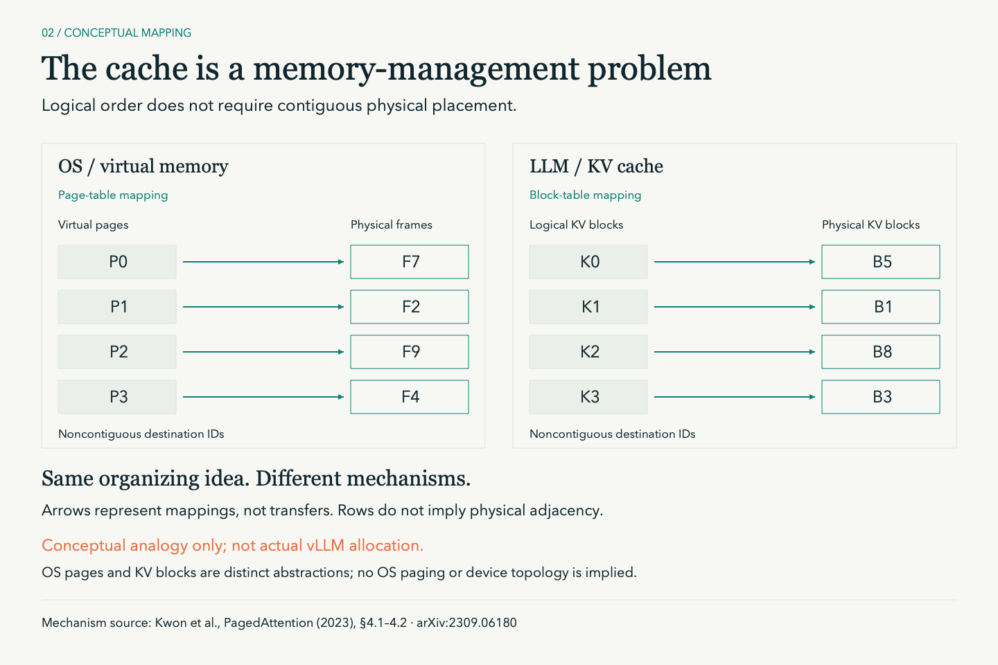
PagedAttention makes the historical connection explicit. Its authors describe an attention algorithm inspired by operating-system virtual memory and paging. Logical KV blocks map to physical blocks that need not be contiguous, with allocation and sharing managed at block granularity.7

OS paging and PagedAttention both separate a logical sequence from its physical placement. The labels are illustrative; this is an abstraction comparison, not an implementation trace. Original illustration based on the PagedAttention paper.7

Memory efficiency affects how many requests can remain active. Sharing can avoid duplication where the model inputs and implementation permit it. Preemption introduces a choice about preserving state or paying to recreate it.7

Track cache occupancy alongside the request mix, including long contexts and periods of overload. Check that abandoned requests release their state after cancellation. Verify how prefix reuse works in the implementation you operate; similar-looking prompts do not, by themselves, establish that the cached state can be shared.

Disaggregation puts the network on the critical path

Prefill processes the prompt and establishes the initial attention state. Decode extends the sequence through successive output tokens. The phases place different demands on the serving system, and colocating them can create interference.8

DistServe separates prefill and decode onto different GPUs and chooses resource allocation and placement around latency requirements and available bandwidth.8

Separating the phases requires moving the relevant KV state, and DistServe's placement strategy accounts for that transfer.8 Whether the split helps your service depends on the workload and the infrastructure connecting the pools.

Test a colocated baseline before adding separate pools. Compare prompt lengths, concurrency and latency under equivalent resource budgets. Include transfer time and queuing. A faster prefill stage does not justify an architecture that delays decode enough to make the request slower.

Engineers who have worked with disaggregated infrastructure will recognize the tradeoff: separate pools can scale independently, but they add coordination and data movement.

Measure the service, then choose the optimization

In The Tail at Scale, Jeffrey Dean and Luiz André Barroso describe how latency variability becomes harder to contain as systems grow and utilization rises.9 Inference gives operators another reason to take that lesson seriously: each additional queue, model pool or state transfer can affect request completion.

Use a fixed evaluation procedure before combining optimizations:

• Define the workload. Record prompt lengths, expected output lengths, arrival patterns, context limits and the task-quality tests. Include difficult requests and bursts.
• Set service targets. Measure latency from the client's initial submission, including queues, routing and retries. Specify acceptable time to first delivered token, response completion time and output quality. For streaming, report gaps between output-bearing events separately from average time per generated token, and state how you calculate that average. Speculative decoding can produce several tokens per target-model pass; delivery cadence need not match token generation.4
• Establish a baseline. Measure the complete request path under realistic concurrency. Retain latency distributions rather than reporting only averages.
• Change one mechanism. Compare equivalent workloads and resource budgets. Include draft-model work, cache transfers, routing, retries and failures where applicable.
• Test overload and cancellation. Observe queue growth, rejected work, resource release and recovery when demand falls.

For this evaluation, define goodput as qualifying logical requests completed per second. Each must pass the task-quality checks and meet the latency targets. Count each original request once, regardless of retries or fallback calls. Report offered load, failures and rejections alongside goodput.

Declare a measurement window with a consistent warm-up and drain policy. Report outstanding requests at the boundary and account for the work needed to resolve them. Separate explicit user cancellations from deadline expirations and service failures. Cancelled requests do not count as qualifying completions, but their consumed resources remain in the cost calculation. Keep that policy consistent across comparisons.

For cost per qualifying request, divide the declared serving cost by qualifying logical requests. Include provisioned resources across all serving stages, including idle capacity, routing, draft models and transfers. State whether model preparation and ongoing evaluation costs are excluded or amortized separately. A lower bill achieved by silently dropping difficult work is not an improvement.

This is a suggested evaluation procedure. No serving benchmark was conducted for this article.

Start with the measured constraint. If weight storage prevents deployment, evaluate quantization. If active sequence state limits concurrency, inspect KV allocation. If mixed request lengths cause avoidable waiting, examine scheduling. Use speculation, distillation or phase separation only when their additional work and operating complexity earn a measurable return.

Experience with networks and distributed systems is useful here. It helps teams recognize when a promising component-level improvement has moved the bottleneck somewhere else. The models have changed, but requests still queue, memory still fills and data still takes time to move. There is no reason to learn all of those lessons again from scratch.

Sources

• [1] Orca: A Distributed Serving System for Transformer-Based Generative Models
• [2] Least Squares Quantization in PCM
• [3] GPTQ: Accurate Post-Training Quantization for Generative Pre-trained Transformers
• [4] Fast Inference from Transformers via Speculative Decoding
• [5] Model Compression
• [6] Distilling the Knowledge in a Neural Network
• [7] Efficient Memory Management for Large Language Model Serving with PagedAttention
• [8] DistServe: Disaggregating Prefill and Decoding for Goodput-optimized Large Language Model Serving
• [9] The Tail at Scale
• [10] SEDA: An Architecture for Well-Conditioned, Scalable Internet Services

Until next time, protect yourselves and safeguard each other